Three-Dimensional Line Tracing
These scripts allow for the tracing of lines embedded in s4d volumes, offering one option which is automated but less reliable, and one which is more robust but requires user input. This documentation walks through the required modules, explains how each of the scripts works, and demonstrates example usage on some included test data.
Contents and Dependencies
Tracing scripts are accessible via the git server. The folder also includes sample data to test each script on. To download the code, run the following command (this will require a log-in to the Git server):
$ git clone ssh://<YOUR_NAME>@immenseirvine.uchicago.edu/git/tracing
The cloned folder should contain the two scripts used to launch the path tracing:
- trace_paths_automated.py
- trace_paths_guided.py
The first script traces the paths in a volume without requiring any user input; however, based on the quality of the data this process may fail for frames even when the path is perhaps distinguishable by eye. The second script is meant to cover those cases where the first script fails, by selecting a handful of problematic frames and allowing the user to interact with the tracing process to improve the chance of a positive outcome.
Additionally, the folder will contain a number of codes, directories, and modules needed to successfully execute the above scripts. Prior to running the scripts, you’ll need a number of in-house, all of which are contained within the ILPM package:
- vector
- path
- networks
The first two modules assist in handling the paths as they are traced, while the last is used to quickly determine distances between collections of points. The last piece of software you’ll need is a command line tool known as UNU, which is needed for the ridge extraction process responsible for finding unordered points that lie on line-like features in the volume. To download and install both ILPM and UNU, see the Module Installation section below.
Module Installation
ilpm package
To download the ILPM package, simply check it out from the git repo and use the setup.py file to install it:
$ git clone ssh://<YOUR_NAME>@immenseirvine.uchicago.edu/git/ilpm
$ cd ilpm
$ sudo python setup.py develop
After doing so, you should have global access to the modules contained in the package. You can your access to vector, path, and networks modules by navigating to a directory that does not contain the ILPM folder, entering a python environment and typing:
from ilpm import vector, path, networks
If no error is returned, the installation was successful and you now have access to all ILPM modules using the same import syntax.
UNU
Instructions for downloading and installing UNU can be found here: http://teem.sourceforge.net/build.html. When configuring the build, be sure to select these options if available in the current build:
- turn “ON” BUILD_EXPERIMENTAL_LIBS
- turn “ON” BUILD_EXPERIMENTAL_APPS
- turn “ON” BUILD_SHARED_LIBS
- turn “ON” Teem_PNG and Teem_ZLIB
More documentation on UNU, including the command line functions available in the package, can be found here: http://teem.sourceforge.net/unrrdu/.
Required Directories and Files
Since line tracing is likely the first process to be executed on a particular experiment, little is required in terms of existing files. The minimal requirements are:
- The sparse file for the experiment
- The S4D for that sparse file
- A directory named with the date (YYYY_MMM_DD) containing the encoder read-out
Note that each of the test data directories contain exactly this information. Prior to executing any tracing scripts, you’ll have to process the information generated by the encoder using the script contained in the tracing dir, for example:
$ python process_encoder_speeds.py ./test_data_1/2015_05_12
After that, the automated tracing algorithm can be executed on the data, followed by the guided version. See the Example Usage section below for more information on executing the scripts.
Tracing Process, Step-by-step
The tracing is designed as a two step process, where the first step is completely automated, tracing a good chunk of the experiment, while the second step then uses user input to assist in tracing the volumes that were not successfully traced by the automated script.
Step 1: Automated Tracing with connect_points_automated.py
Ridge Extraction
The first step in tracing the paths is to identify points in space that likely lie on the path. This is accomplished via a process known as ridge extraction, in which particles that have interaction potentials both with each other and with the background intensity are seeded in the volume and allowed to relax to a configuration where they are aggregated along line-like features. After parsing which frames need to be ridge extracted, the call to the UNU functions is made via a python function, as shown below
#PARSE WHETHER OR NOT THE FRAMES ARE THE SAME FOR EACH SPARSE FILE
if len(args.frames)==1 and len(args.input)!=1:
        sys.exit('Number of input sparse files does not match number of frames options')
frame_set = []
for frame_string in args.frames: frame_set.append(eval('x[%s]'%frame_string, {'x': range(1000)}))

#CHECK TO SEE WHICH FRAMES ALREADY HAVE POINTS AND WHICH NEED TO BE PROCESSED
for sparse_file, frames in zip(sparse_files, frame_set):
        if ridgeOverwrite: missing_frames = frames
        else:
                missing_frames = []
                for f in frames:
                        if not check_for_pts(sparse_file, f): missing_frames.append(f)
        #RUN RIDGE EXTRACTION ON THE MISSING FRAMES
        if len(missing_frames)!=0: ridge_extract_by_frames(sparse_file, missing_frames)
The final line, containing the call to ridge_extract_by_frames, will iteratively run the script cp_ridge_extraction.py for each of the desired frames. After this process is complete, a subdirectory called points should be generated in which .txt files of the (x,y,z) coordinates are stored for each frame. Snapshots of the points will also be stored in the pngs subdirectory.
Point Linking
The points from the ridge extraction process are not ordered, do not necessarily cover the entire vortex, and are not guaranteed to lie on the vortex if there are errant line-like structures in the volume. As such, a fair amount of processing must be accomplished to turn these points into closed paths. The first step is to make connections between points based on the number and proximity of their neighbors. Once equilibrated, the ridge extraction process will return points that have a characteristic spacing, which can then be used to determine how many neighbors each point has within that distance. Starting with points that have only one neighbor (and thus represent the possible terminus of a line segment), points are iteratively added to the ends of growing lines. This is accomplished by calling:
X = loadtxt(open(os.path.join(points_dir, point_fn)), usecols=range(3))
D = make_dist_table(X)
neighbors, visited = assign_neighbors(D)
lines_ids = connect_points(D, neighbors)
Line Filtering
The result from the point-linking process will be a collection of line segments. Some of these segments will be errant, and the ends of even correct segments might contain a few errant points. To avoid mistakes due to shorter off-path lines and wiggly ends, the line segments are filtered, tossing out lines that contain fewer than LENGTH_TOLERANCE points, and eroding ERODE_AMOUNT from both sides. This is accomplished by calling a single function:
lines_ids = filter_lines_ids(lines_ids)
Gap Filling
There will be gaps between the ends of the line segments that need to be filled, which ultimately is accomplished by fast-marching between the end points of two existing line segments. In order to accomplish this, the end points which should be connected need to first be identified. These pairings are determined by generating a distance map for each end point that shows how connected that point is to every other point in space by bright lines in the volume. Points which are mutually closest to each other in this distance map are paired, and the line connecting them is generated by climbing the gradient of the distance map from the target to the source. Again, this is accomplished by a single function call:
lines_xyz = fast_march_gaps(raw_data, X, lines_ids)
Path Annealing
The result of fast marching will still be a collection of line segments, but now many of them should share end points, allowing them to be connected into loops. Line segments that are not part of closed loops are discarded. The number of loops is then compared against the target number specified by path_number; if the number is greater than path_number, only the longest path_number loops will be preserved. NOTE that for vortices where the path number increases through reconnection, the two sections of the video will have to be processed independently, or path_number must be set to the largest number of expected loops. This entire process is two function calls:
loops_xyz = anneal_paths(lines_xyz)
loops_xyz = remove_additional_loops(loops_xyz, path_number)
Saving and Reporting
When tracing an experiment, a log is generated to keep track of which frames have been attempted and whether or not the tracing for that frame was successful. If no closed loops are found, then the script will record the status of that frame as “bad” in the log and move on to the next frame. If closed loops are found, it will save a snapshot of those loops overlaid on a projection of the experimental volume, and record the total path length for that frame in the log.
if not loops_xyz:
        update_log(sparse_file, f, 'frames', 'bad')
        print 'No Closure Path Found'

else:

        save_snapshot(s4d, f, loops_xyz, sparse_file)
        loops_xyz = perspective_correct(loops_xyz, setup_info)
        save_trace(f, loops_xyz, setup_info, sparse_file)

        print 'Closed path traced for frame ', f

        total_length = get_total_loop_length(loops_xyz)
        update_log(sparse_file, f, 'length', total_length)
Once all the frames have been traced, the code will look for path lengths that differ dramatically from the mean length and label them “bad” frames in an effort to identify frames where the closed loops were found but for which there are still issues.
Step 2: Guided Tracing with connected_points_guided.py
Frame Selection
Once the automated code has been run, there will likely be some number of frames that were successfully traced, and some (hopefully smaller!) number that were not. connected_points_guided.py is meant to trace those frames that the automated script could not. The first step in this process is to find the frames that need to be processed. This can be set manually by including the optional command line argument -frames when executing the script; if this option is omitted, it will set frames to be all those that were marked as “bad” in the log, either because they contained no closed loops or because the total length of the collection of loops seemed significantly different from the rest of the frames.
#CHECK TO SEE WHICH FRAMES NEED TO BE PROCESSED
points_dir = get_sparse_subdir(sparse_file, 'points')
if frames is None:
        frames = grab_bad_frames(sparse_file)
        print frames
        point_fns = get_points(sparse_file, points_dir, frames)
else:
        frames = eval('x[%s]' % args.frames, {'x': range(1000)})
        point_fns = get_points(sparse_file, points_dir, frames)
Point Linking and Line Filtering
The script begins in the same way as the automated version. See the two sections above for more detail about how the initial line segments are determined from the ridge points.
Line Culling
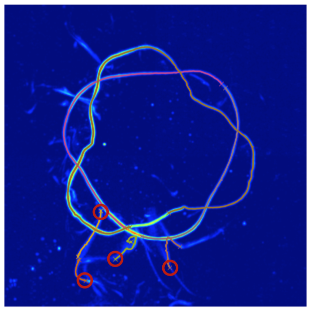
Once the initial line segments have been established, the script gives the user a chance to delete segments they believe to be errant. A figure will pop up showing a projection of the data along with all the current line segments with their end points marked by ‘x’. By clicking near one of the two end points of a segment, you can exclude that segment from future consideration.
lines_ids = remove_bad_lines(raw_data, X, lines_ids)
Directed Fast Marching
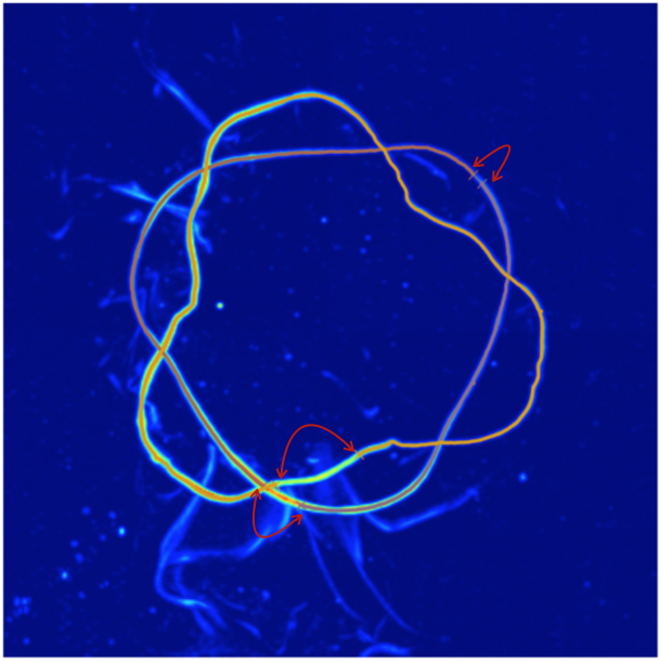
Instead of letting the code determine which end points should be connected via fast marching, the guided script again prompts the user to indicate these connections manually. A figure will pop up showing the remaining line segments again with their end points marked by ‘x’. Sequentially click on the pairs of end points that should be connected (order within a pair does not matter). All endpoints must be clicked on, so it’s important that you removed all paths you don’t want in the previous step.
lines_xyz = fast_march_gp_gaps(raw_data, X, lines_ids)
Path Annealing, Saving, and Reporting
The final steps of the process are the same as in the automated case, see above for more detail.
Example Usage on Test Data
Test Data 1: Isolated Helix
On labshared2 there is a directory called test_data that contains two subdirectories line_tracing_1 and line_tracing_2 which contain sample data sets for the tracing algorithms. The first set of test data is of an isolated helix imaged using dye. For a simple geometry and a good dye job, this should be an easy thing to track. To get started, confirm that this directory has everything you need: a sparse, an s4d, and encoder information:
$ /Volumes/labshared2/test_data/line_tracing_1/2015_05_12/
$ /Volumes/labshared2/test_data/line_tracing_1/2015_05_12_THL001_psi40_spacer7_filter_over_solohelix_eye_IV.sparse
$ /Volumes/labshared2/test_data/line_tracing_1/2015_05_12_THL001_psi40_spacer7_filter_over_solohelix_eye_IV.s4d
The first step is to process the cart speeds recorded by the encoder, so we’ll run:
$ python process_encoder_speeds.py /Volumes/labshared2/test_data/line_tracing_1/2015_05_12/
Next we’ll attempt to do some number of frames, say numbers 20 through 25 using the automated code. To launch this, simply type:
$ python connect_points_automated.py /Volumes/labshared2/test_data/line_tracing_1/2015_05_12_THL001_psi40_spacer7_filter_over_solohelix_eye_IV.sparse -frames 20:26 -path_number 1
There are four command line arguments for this script:
- -frames: The frames to be processed in standard python slice notation. The number of arguments here must either be one or the number of sparse file inputs. Default = None.
- -path_number: The expected maximal number of paths throughout the entire experiment. Default = 10.
- –overwrite: If included, will overwrite previously traced paths using the existing ridge extraction data. Default = False.
- –ridgeOverwrite: Overwrite the previously extracted ridge points. Default = False.
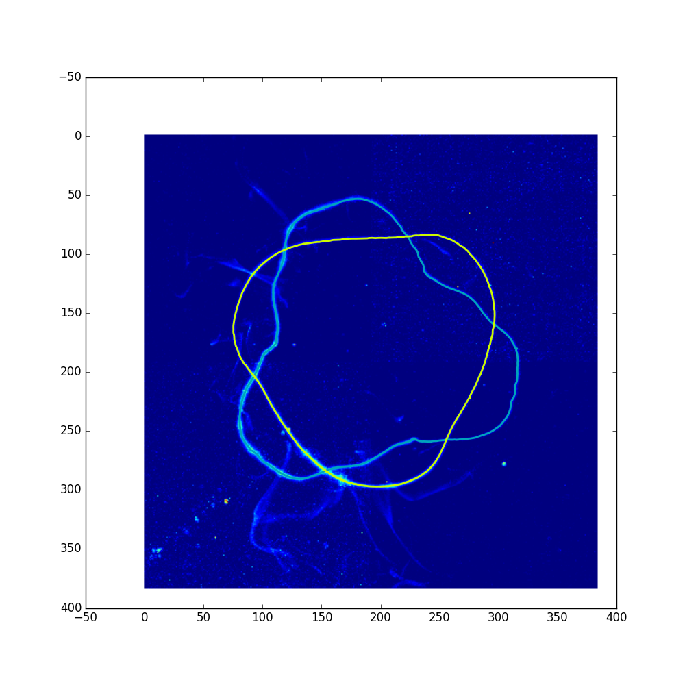
Note that because we have an isolated helix that we know doesn’t undergo reconnection, we have no problem setting the path number to 1. Following this process, you should have a new directory named after the sparse file that has paths and path_proj subdirectories. The first stores the traced paths as .json files while the second contains snapshots of the results useful for diagnosing the tracing. The snapshot for frame number 20 is included below:
There will also be a new .json file in the test_data_1 directory, which is the log that keeps track of which frames have been attempted and whether or not they were successful. This is human readable, and if you open it you’ll see that each frame has been labeled as “good” for this tracing, since the script was able to find a closed loop with a reasonable length for all the frames considered. In this case, no additional tracing is needed.
Test Data 2: Re-knotting Loops
The second set of data is a little more complex than the first: it contains two loops which are leap-frogging as they approach a series of reconnection events that will briefly form a knot. The presence of multiple paths, errant dye wisps, and topology changes make this a potentially problematic experiment to trace. Never the less, we’ll begin again by processing the encoder information:
$ python process_encoder_speeds.py /Volumes/labshared2/test_data/line_tracing_2/2017_01_17
Next we’ll again attempt to automatically trace frames 20 through 25. This time, we’ll set the path_number to be 2, which we know is the largest number of loops we’d ever expect throughout the entire experiment. To execute, we type:
$ python connect_points_automated.py /Volumes/labshared2/test_data/line_tracing_2/2017_01_17_FFP002_dye_psi70_II.sparse -frames 20:26 -path_number 2
Again, a directory and log for this experiement will be generated, and inside the paths and path_proj subdirectories will be the results of the tracing. Opening up the path_proj directory, you’ll notice that frame 21 has only one of the two paths traced, and as such, it is marked as “bad” in the log. The projection of this frame is shown below
To fix this, the guided version can be used. To launch it, type:
$ python connect_points_guided.py /Volumes/labshared2/test_data/line_tracing_2/2017_01_17_FFP002_dye_psi70_II.sparse
This method has only one additional command line argument -frames, which indicates which frames are to be processed. While the automated script requires some frames be specified, omitting frames for the guided version will direct the code to try and process any frame that are labeled “bad” in the log.
Since we’ve omitted the -frames argument, this will attempt to re-trace any frames that were labeled as “bad”. Two windows will pop up during this process, the first will allow you to remove the errant lines by clicking on one of their end points (you must remove all errant lines). The figure below shows possible clicks you could make to remove these lines.
The second window will allow you to indicate which end points should be connected (you must pair all remaining end points). The figure below shows pairs of points that should be clicked sequentially. The order inside any pair does not matter, nor does the order of the pairs.
Once the script is done running, check the path_proj subdirectory to see that now both paths appear in the trace, and check the log to see that the status has been updated to “good” to reflect this correction.


